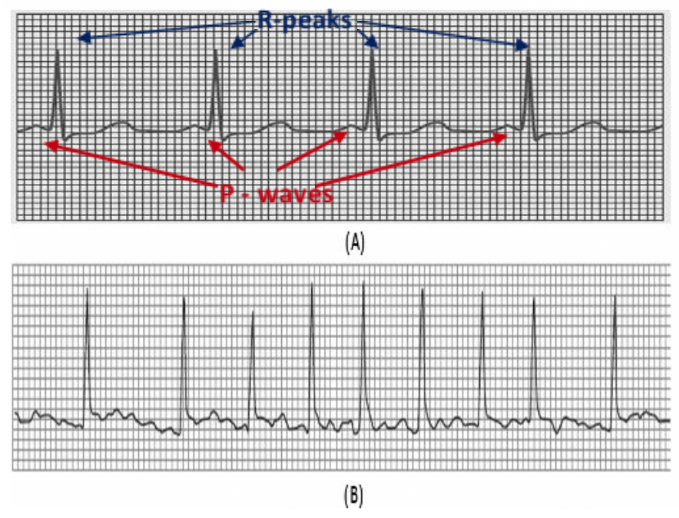
Cardiac arrhythmias are disorders in the electrical activity of the heart characterised by fast or slow beats often accompanied by an irregular rhythm pattern. In addition, some arrhythmias exhibit morphological changes in the electrocardiogram (ECG) as a result of damage of heart cells and abnormal conduction of the impulses. Some arrhythmias are benign, and others are life-threatening or may lead to severe health complications. Atrial fibrillation (AF) belongs to the latter category; and it is characterised by irregular R-R intervals, and fluttering activity instead of P-waves as a result of the abnormal activity of the atrium (figure 1). AF may lead to severe life-threatening events (such as stroke) when left untreated. In addition, AF is the most common arrhythmia affecting many people around the globe.

Detecting arrhythmias such as AF is not something novel; and in fact, most of medical bedside monitors and cardiac telemetry systems have capabilities for arrhythmia detection. Nevertheless, detecting arrhythmia using wireless wearable devices – i.e. where not only the ECG morphology can be affected by motion artefacts, but also the rhythm can be altered by the intensity of physical activity – is still challenging. Here we present a simple method to detect atrial fibrillation on patients with no other comorbidities and who may or may not have been diagnosed with this arrhythmia (but who could be at risk or presenting with symptoms). This approach is based on the analysis of the regularity and speed of the rhythm only. We used real, accredited and annotated ECG data from MIT-BIH Arrhythmia and AF databases available in www.physionet.org. The ECG records were segmented into epochs of 30 seconds of duration. Thus, the data was partitioned such that 2900 samples (80%) were used for training and 726 (20%) for testing.
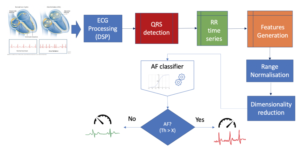
Figure 2 portrays the logic of the algorithm. First ECG segments are filtered to remove noise from different sources affecting the quality of the data (e.g. mains interference, motion artefacts, baseline wandering and high-frequency noise). Subsequently, the epochs are processed by an algorithm that detects the heart beats (R-peaks) based on different mathematical and physiological characteristics of incoming ECG segments. The outcome of the algorithm are time series of R peaks positions and amplitudes, as well as a time series of R-R intervals corresponding to the current segment. This information is then crunched using statistical and signal processing methods to obtain a set of values describing a number of features of each segment. Thus, each ECG epoch is basically converted into a multidimensional vector (or point) in a feature space. The resultant feature space is normalised between 0 and 1 to minimise optimisation bias during the training process.
We initially generated input vectors formed by more than 20 selected features generated from the time series of R-peaks and RR intervals. However, high dimensionality of the resultant feature space often lead to the following issues:
- Complex models and large size datasets that are computationally expensive in terms of processing and storage (curse of dimensionality). In addition, high dimensional classification algorithms are often difficult to implement in wearable devices, particularly when there are limitations in terms of processing and power consumption (i.e. battery life).
- Complexity does not imply effectiveness – i.e. highly dimensional features spaces often contain irrelevant information that can introduce confounding factors leading to larger classification errors and limited ability to generalise when processing unseen data.
Therefore, a crucial part of the approach discussed in this post is about reducing the dimensionality of the feature space as much as possible to simplify the algorithm and minimise the size of the dataset. For such a purpose we applied an unsupervised algorithm that applies a linear transformation to find orthogonal projections of the original data in a lower dimensional space – i.e. in simple terms, Principal Component Analysis (PCA) is a technique that searches for the directions of largest variance of the high-dimensional dataset and projects it into a new subspace with less dimensions than the original one. The ultimate goal is to construct a o x n-dimensional transformation matrix W that is used to map the original input vectors into a new subspace with less dimensions than the original. Thus, for each observation of the original feature space:

Where x = [x1, x2, …, xo] is the original o-dimensional input vector, and z = [z1, z2, …, zn] is the new n-dimensional vector projected in the new lower-dimensional space. Note that o >>> n. For a new n-dimensional feature space, building the matrix involve the following steps:
- Center the data by subtracting the mean from the dataset.
- Calculate the covariance matrix.
- Decompose the covariance matrix into its eigenvectors and eigenvalues.
- Select the n-eigenvectors corresponding with the largest n-eigenvalues (components with the largest variance) corresponding to the n-dimensions of the new feature space.
- Construct the transformation matrix W using these n-eigenvectors.
- Apply the transformation to each observation of the original dataset (see equation 1) to obtain (or map a single input vector to) the new n-dimensional feature space.
In our particular case, the 20-dimensional original feature space was transformed into a 2-dimensional feature space projected along the principal components of the data (figure 2). The number of new dimensions n where such that the minimum total variance explained by the selected components is equal or greater than a certain threshold. For illustration purposes, we chose 2 components for a total variance threshold of 85%. In a real application, 5 components will account for >95% of the variance.

Input vectors from the new feature space are then fed into a classifier that predicts the probability of AF. Here we trained to simple classifiers. The first one was a Gaussian Naïve Bayes classifier, which assumes that the input data is drawn from a normal distribution. Thus, classification is derived from the Bayes’s rule as follows:
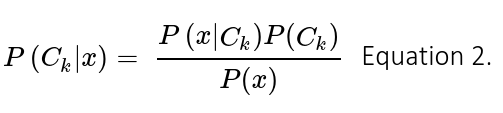
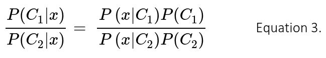
Where Ck is the k-class, and x the input vector of features. In this binary classification problem k = 2 and hence the classification decision is given by the ratio of posterior probabilities for each label:
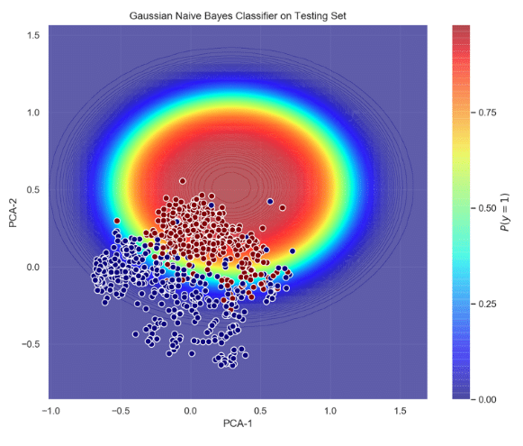
Training this classifier involves estimation of the generative model that hypothetically corresponds to the random process that generates the data. Typically, finding the model that best represents the data is a complicated task. However, we naively assumed that the data the data follows a Gaussian distribution – i.e. this is where the term ‘naïve’ stems from. Figure 3 shows the probabilistic decision function of the gaussian classifier acting on the testing set, and its ROC curve. It can be seen that the probability of AF increases as the datapoints move towards the center of the ellipse (red area); and most of the AF points lie inside the ellipse. This good separability is confirmed by the area under the curve (AUC = 0.97), true positive rate (tpr = 0.94) and false positive rate (fpr = 0.14).
Although the accuracy of this classifier is good for this dataset, we went one step ahead in trying to model the actual distribution of the data. Therefore, we implemented another Bayesian Classifier using Kernel Density Estimation (KDE) to find the probability density functions (pdfs) that best represented the data. When using KDE one can estimate the density function p(x) to find the probability of any sample corresponding to a specific class in the feature space. Following the application of some probability theory and maths (out of the scope of this article), the shape of the pdf for a multivariate is then estimated using the following expression:

Where K is the kernel (positive and symmetric function which area under the curve equals to 1); d the number of dimensions of the feature space; x the average (or central) point at which KDE is performed for any xi point; and h is the bandwidth that serves as a smoothing parameter that controls kernel’s size at each point . Training KDE models focuses on implementing the right kernel and finding the optimal value for h based on minimization of a cost functions (e.g. L2 risk function or mean integrated square error – MISE); thus, machine learning pipelines using grid searches and cross-validation to select the best kernel and bandwidth value for the final implementation of the model.
There are different kernels available, being the Gaussian kernel the most popular one. After embedding the Gaussian kernel into equation 4 we have:
Finally, the steps for Bayesian classification using generative models from KDE are:
- Stratify and divide the training dataset into partitions grouped by class.
- Apply KDE to each partition to obtain the generative model corresponding to each class. This makes possible computation of the conditional probability P(x|Ck), or likelihood of class k for any observation x.
- Compute the prior probabilities P(Ck) for group of samples corresponding to each class k.
- Lastly, once the classifier is trained, a new prediction can be made for any unseen point x by calculating the posterior probability P(Ck|x)∝P(x|Ck)P(Ck) for each class k. Thus, the class with the highest probability is assigned to the current point x.
Figure 4 shows the decision function and the ROC curve for this Bayesian KDE classifier. It can be seen that the accuracy of this classifier is slightly higher than the previous one – i.e. tpr = 0.96.

In summary, this post presented methods to develop low-dimensional probabilistic algorithms for classification of ECG arrhythmias. It is important to bear in mind that these examples are only illustrative and therefore a larger and more representative dataset that includes other conditions and noisy signals might be necessary to retrained/tune these classifiers or develop new ones, suitable for integration in wearable products.